Discrete choice
In economics, discrete choice problems involve choices between two or more discrete alternatives, such as entering or not entering the labor market, or choosing between modes of transport. Such choices contrast with standard consumption models in which the quantity of each good consumed is assumed to be a continuous variable. In the continuous case, calculus methods (e.g. first-order conditions) can be used to determine the optimum, and demand can be modeled using regression analysis. On the other hand, discrete choice analysis examines situations in which the potential outcomes are discrete, such that the optimum is not characterized by standard first-order conditions. Loosely, regression analysis examines “how much” while discrete choice analysis examines “which.” However, discrete choice analysis can be and has been used to examine the chosen quantity in particular situations, such as the number of vehicles a household chooses to own [1] and the number of minutes of telecommunications service a customer decides to use.[2]
Discrete choice models are statistical procedures that model choices made by people among a finite set of alternatives. The models have been used to examine, e.g., the choice of which car to buy,[1][3] where to go to college,[4] , which mode of transport (car, bus, rail) to take to work[5] among numerous other applications. Discrete choice models are also used to examine choices by organizations, such as firms or government agencies. In the discussion below, the decision-making unit is assumed to be a person, though the concepts are applicable more generally. Daniel McFadden won the Nobel prize in 2000 for his pioneering work in developing the theoretical basis for discrete choice.
Discrete choice models statistically relate the choice made by each person to the attributes of the person and the attributes of the alternatives available to the person. For example, the choice of which car a person buys is statistically related to the person’s income and age as well as to price, fuel efficiency, size, and other attributes of each available car. The models estimate the probability that a person chooses a particular alternative. The models are often used to forecast how people’s choices will change under changes in demographics and/or attributes of the alternatives.
Contents
|
Applications
- Marketing researchers use discrete choice models to study consumer demand and to predict competitive business responses, enabling choice modelers to solve a range of business problems, such as pricing, product development, and demand estimation problems.[1]
- Transportation planners use discrete choice models to predict demand for planned transportation systems, such as which route a driver will take and and whether someone will take rapid transit systems.[5][6] The first applications of discrete choice models were in transportation planning, and much of the most advanced research in discrete choice models is conducted by transportation researchers.
- Energy forecasters and policymakers use discrete choice models for households’ and firms’ choice of heating system, appliance efficiency levels, and fuel efficiency level of vehicles.[7][8]
- Environmental studies utilize discrete choice models to examine the recreators’ choice of, e.g., fishing or skiing site and to infer the value of amenities, such as campgrounds, fish stock, and warming huts, and to estimate the value of water quality improvements.[9]
- Labor economists use discrete choice models to examine participation in the work force, occupation choice, and choice of college and training programs.[4]
Common Features of Discrete Choice Models
Discrete choice models take many forms, including: Binary Logit, Binary Probit, Multinomial Logit, Conditional Logit, Multinomial Probit, Nested Logit, Generalized Extreme Value Models, Mixed Logit, and Exploded Logit. All of these models have the features described below in common.
Choice Set
The choice set is the set of alternatives that are available to the person. For a discrete choice model, the choice set must meet three requirements:
- The set of alternatives must be exhaustive, meaning that the set includes all possible alternatives. This requirement implies that the person necessarily does choose an alternative from the set.
- The alternatives must be mutually exclusive, meaning that choosing one alternative means not choosing any other alternatives. This requirement implies that the person chooses only one alternative from the set.
- The set must contain a finite number of alternatives. This third requirement distinguishes discrete choice analysis from regression analysis in which the dependent variable can (theoretically) take an infinite number of values.
- Example: The choice set for a person deciding which mode of transport to take to work includes driving alone, carpooling, taking bus, etc. The choice set is complicated by the fact that a person can use multiple modes for a given trip, such as driving a car to a train station and then taking train to work. In this case, the choice set can include each possible combination of modes. Alternatively, the choice can be defined as the choice of “primary” mode, with the set consisting of car, bus, rail, and other (e.g. walking, bicycles, etc.). Note that “other” alternative is used to make the choice set exhaustive.
Different people may have different choice sets, depending on their circumstances. For instance, Toyota-owned Scion is not sold in Canada as of 2009, so new car buyers in Canada face different choice sets from those of American consumers.
Defining Choice Probabilities
A discrete choice model specifies the probability that a person chooses a particular alternative, with the probability expressed as a function of observed variables that relate to the alternatives and the person. In its general form, the probability that person n chooses alternative i is expressed as:

where
 is a vector of attributes of alternative i faced by person n,
 is a vector of attributes of the other alternatives (other than i) faced by person n,
 is a vector of characteristics of person n, and
 is a set of parameters that relate variables to probabilities, which are estimated statistically.
In the mode of transport example above, the attributes of modes (xni), such as travel time and cost, and the characteristics of consumer (sn), such as annual income, age, and gender, can be used to calculate choice probabilities. The attributes of the alternatives can differ over people; e.g., cost and time for travel to work by car, bus, and rail are different for each person depending on the location of home and work of that person.
Properties:
-
- Pni is between 0 and 1
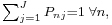 where J is the total number of alternatives.
- Expected share choosing i
 where N is the number of people making the choice.
Different models (i.e. different function G) have different properties. Prominent models are introduced below.
Consumer Utility
Discrete choice models can be derived from utility theory. This derivation is useful for three reasons:
- It gives a precise meaning to the probabilities Pni
- It motivates and distinguishes alternative model specifications, e.g., G’s.
- It provides the theoretical basis for calculation of changes in consumer surplus (compensating variation) from changes in the attributes of the alternatives.
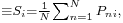
Uni is the utility (or net benefit or well-being) that person n obtains from choosing alternative i. The behavior of the person is utility-maximizing: person n chooses the alternative that provides the highest utility. The choice of the person is designated by dummy variables, yni, for each alternative:
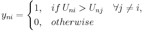
Consider now the researcher who is examining the choice. The person’s choice depends on many factors, some of which the researcher observes and some of which the researcher does not. The utility that the person obtains from choosing an alternative is decomposed into a part that depends on variables that the researcher observes and a part that depends on variables that the researcher does not observe. In a linear form, this decomposition is expressed as
where
 is a vector of observed variables relating to alternative i for person n that depends on attributes of the alternative, xni, interacted perhaps with attributes of the person, sn, such that it can be expressed as
-
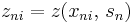 for some numerical function z,
-
 is a corresponding vector of coefficients of the observed variables, and
 captures the impact of all unobserved factors that affect the person’s choice.
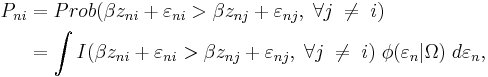
The choice probability is then
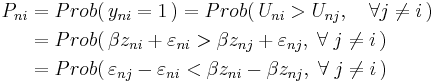
Given β, the choice probability is the probability that the random terms, εnj − εni (which are random from the researcher’s perspective, since the researcher does not observe them) are below the respective quantities 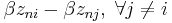 . Different choice models (i.e. different specifications of G) arise from different distributions of εni for all i and different treatments of β.
Properties of Discrete Choice Models Implied by Utility Theory
Only differences matter
The probability that a person chooses a particular alternative is determined by comparing the utility of choosing that alternative to the utility of choosing other alternatives:
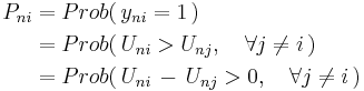
As the last term indicates, the choice probability depends only on the difference in utilities between alternatives, not on the absolute level of utilities. Equivalently, adding a constant to the utilities of all the alternatives does not change the choice probabilities.
Scale must be normalized
Since utility has no units, it is necessary to normalize the scale of utilities. The scale of utility is often defined by the variance of the error term in discrete choice models. This variance may differ depending on the characteristics of the dataset, such as when or where the data are collected. Normalization of the variance therefore affects the interpretation of parameters estimated across diverse datasets.
Prominent Types of Discrete Choice Models
Discrete choice models can first be classified according to the number of available alternatives.
- * Binomial choice models (dichotomous): 2 available alternatives
- * Multinomial choice models (polytomous): 3 or more available alternatives
Multinomial choice models can further be classified according to the model specification:
- * Models, such as standard logit, that assume no correlation in unobserved factors over alternatives
- * Models that allow correlation in unobserved factors among alternatives
In addition, specific forms of the models are available for examining rankings of alternatives (i.e., first choice, second choice, third choice, etc.) and for ratings data.
Details for each model are provided in the following sections.
Binary Choice
A. Logit with attributes of the person but no attributes of the alternatives
Un is the utility (or net benefit) that person n obtains from taking an action (as opposed to not taking the action). The utility the person obtains from taking the action depends on the characteristics of the person, some of which are observed by the researcher and some are not:
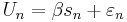
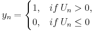
The person takes the action, yn = 1, if Un > 0. The unobserved term, εn , is assumed to have a logistic distribution.
The specification is written succinctly as:
-
- Un = βsn + εn
- ε ∼ Logistic,
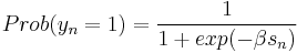
Then the probability of taking the action is
B. Probit with attributes of the person but no attributes of the alternatives
The description of the model is the same as model A, except the unobserved terms are distributed standard normal instead of logistic.
-
- Un = βsn + εn
- ε ∼ Standard normal,
Then the probability of taking the action is
-
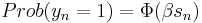 ,
,- where Φ() is cumulative distribution function of standard normal.
C. Logit with variables that vary over alternatives
Uni is the utility person n obtains from choosing alternative i. The utility of each alternative depends on the attributes of the alternatives interacted perhaps with the attributes of the person. The unobserved terms are assumed to have an extreme value distribution.[nb 1]
-
- Un1 = βzn1 + εn1,
- Un2 = βzn2 + εn2,
 iid extreme value,
which gives this expression for the probability
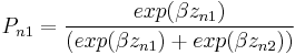
We can relate this specification to model A above, which is also binary logit. In particular, Pn1 can also be expressed as
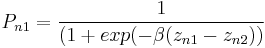
Note that if two error terms are iid extreme value,[nb 1] their difference is distributed logistic, which is the basis for the equivalence of the two specifications.
D. Probit with variables that vary over alternatives
The description of the model is the same as model C, except the unobserved terms are distributed standard normal instead of logistic.
Then the probability of taking the action is
-
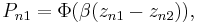
- where Φ is the cumulative distribution function of standard normal.
Multinomial Choice without Correlation Among Alternatives
E. Logit with attributes of the person but no attributes of the alternatives
The utility for all alternatives depends on the same variables, sn, but the coefficients are different for different alternatives:
-
- Uni = βi'sn + εni,
- Since only differences in utility matter, it is necessary to normalize
 for one alternative. Assuming
  ,
, - εni ∼ iid extreme value [nb 1]
The choice probability takes the form
-
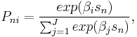
- where J is the total number of alternatives.
F. Logit with variables that vary over alternatives (also called conditional logit)
The utility for each alternative depends on attributes of that alternative, interacted perhaps with attributes of the person:
-
- Uni = βzni + εni,
- εni ∼ iid extreme value,[nb 1]
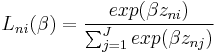
The choice probability takes the form
-
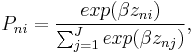
- where J is the total number of alternatives.
Note that model E can be expressed in the same form as model F by appropriate respecification of variables.
-
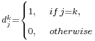
- Let
 be a dummy variable that identifies alternative k:
- Let
-
- Multiply sn from model E with each of these dummies:
 .
. - Then, model F is obtained by using
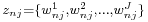 and
and 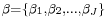 , where J is the number of alternatives.
- Multiply sn from model E with each of these dummies:
Multinomial Choice with Correlation Among Alternatives
A standard logit model is not always suitable, since it assumes that there is no correlation in unobserved factors over alternatives. This lack of correlation translates into a particular pattern of substitution among alternatives that might not always be realistic in a given situation. This pattern of substitution is often called the Independence of Irrelevant Alternatives (IIA) property of standard logit models. See the Red Bus/Blue Bus example [10] or path choice example.[11] A number of models have been proposed to allow correlation over alternatives and more general substitution patterns:
- Nested Logit Model - Captures correlations between alternatives by partitioning the choice set into 'nests'
- Generalised Extreme Value Model[15] - General class of model, derived from the random utility model[11] to which multinomial logit and nested logit belong
- Mixed logit [8][9][17]- Allows any form of correlation and substitution patterns.[18] When a mixed logit is with jointly normal random terms, the models is sometimes called "multinomial probit model with logit kernel"[19] Can be applied to route choice [20]
The following sections describe Nested Logit, GEV, Probit, and Mixed Logit models in detail.
G. Nested Logit and Generalized Extreme Value (GEV) models
The model is the same as model F except that the unobserved component of utility is correlated over alternatives rather than being independent over alternatives.
-
- Uni = βzni + εni,
- The marginal distribution of each εni is extreme value,[nb 1] but their joint distribution allows correlation among them.
- The probability takes many forms depending on the pattern of correlation that is specified. See Generalized Extreme Value.
H. Multinomial Probit
The model is the same as model G except that the unobserved terms are distributed jointly normal, which allows any pattern of correlation and heteroscedasticity:
-
- Uni = βzni + εni,
The choice probability is
-
- where
 is the joint normal density with mean zero and covariance
  .
.
- where
-
- The integral for this choice probability does not have a closed form, and so the probability is approximated by quadrature or simulation.
- When is the identity matrix (such that there is no correlation or heteroscedasticity), the model is called independent probit.
I. Mixed Logit
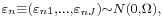
Mixed Logit models have become increasingly popular in recent years for several reasons. First, the model allows β to be random in addition to ε. The randomness in β accommodates random taste variation over people and correlation across alternatives that generates flexible substitution patterns. Second, the advent in simulation has made approximation of the model fairly easy. In addition, McFadden and Train[18] have shown that any true choice model can be approximated, to any degree of accuracy by a mixed logit with appropriate specification of explanatory variables and distribution of coefficients.
-
- Uni = βzni + εni,
 for any distribution
  , where
  is the set of distribution parameters (e.g. mean and variance) to be estimated,
- εni ∼ iid extreme value,[nb 1]
The choice probability is
-
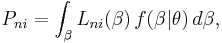
- where
 is logit probability evaluated at
 is the total number of alternatives.
The integral for this choice probability does not have a closed form, so the probability is approximated by simulation. Also see Mixed logit for further details.
Model Applications
The models described above are adapted to accommodate rankings and ratings data.
Ranking of Alternatives
In many situations, a person's ranking of alternatives is observed, rather than just their chosen alternative. For example, a person who has bought a new car might be asked what he/she would have bought if that car was not offered, which provides information on the person's second choice in addition to their first choice. Or, in a survey, a respondent might be asked:
-
- Example: Rank the following cell phone calling plans from your most preferred to your least preferred.
- * $60 per month for unlimited anytime minutes, two-year contract with $100 early termination fee
- * $30 per month for 400 anytime minutes, 3 cents per minute after 400 minutes, one-year contract with $125 early termination fee
- * $35 per month for 500 anytime minutes, 3 cents per minute after 500 minutes, no contract or early termination fee
- * $50 per month for 1000 anytime minutes, 5 cents per minute after 1000 minutes, two-year contract with $75 early termination fee
The models described above can be adapted to account for rankings beyond the first choice. The most prominent model for rankings data is the exploded logit and its mixed version.
J. Exploded Logit
Under the same assumptions as for a standard logit (model F), the probability for a ranking of the alternatives is a product of standard logits. The model is called "exploded logit" because the choice situation that is usually represented as one logit formula for the chosen alternative is expanded ("exploded") to have a separate logit formula for each ranked alternative. The exploded logit model is the product of standard logit models with the choice set decreasing as each alternative is ranked and leaves the set of available choices in the subsequent choice.
Without loss of generality, the alternatives can be relabeled to represent the person's ranking, such that alternative 1 is the first choice, 2 the second choice, etc. The choice probability of ranking J alternatives as 1, 2, …, J is then

As with standard logit, the exploded logit model assumes no correlation in unobserved factors over alternatives. The exploded logit can be generalized, in the same way as the standard logit is generalized, to accommodate correlations among alternatives and random taste variation. The "mixed exploded logit" model is obtained by probability of the ranking, given above, for Lni in the mixed logit model (model I).
This model is also known in econometrics as the rank ordered logit model and it was introduced in that field by Beggs, Cardell and Hausman in 1981[21] · [22]. One application is the Combes et alii paper explaining the ranking of candidates to become professor[22]. Is is also known as Plackett–Luce model in biomedical literature[22].
Ratings Data
In survey, respondents are often asked to give ratings, such as:
-
- Example: Please give your rating of how well the President is doing.
- 1: Very badly
- 2: Badly
- 3: Fine
- 4: Good
- 5: Very good
Or,
-
- Example: On a 1-5 scale where 1 means disagree completely and 5 means agree completely, how much do you agree with the following statement. "The Federal government should do more to help people facing foreclosure on their homes."
A multinomial discrete-choice model can examine the responses to these questions (model G, model H, model I). However, these models are derived under the concept that the respondent obtains some utility for each possible answer and gives the answer that provides the greatest utility. It might be more natural to think that the respondent has some latent measure or index associated with the question and answers in response to how high this measure is. Ordered logit and ordered probit models are derived under this concept.
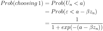
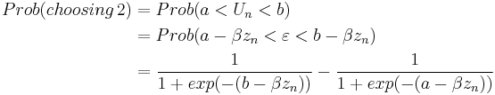
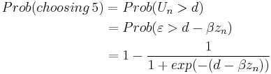
K. Ordered Logit
Let Un represent the strength of survey respondent n’s feelings or opinion on the survey subject. Assume that there are cutoffs of the level of the opinion in choosing particular response. For instance, in the example of the helping people facing foreclosure, the person chooses
- 1, if Un < a
- 2, if a < Un < b
- 3, if b < Un < c
- 4, if c < Un < d
- 5, if Un > d,
for some real numbers a, b, c, d.
Defining 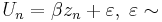 Logistic, then the probability of each possible response is:
and so on up to
The parameters of the model are the coefficients β and the cut-off points a − d, one of which must be normalized for identification. When there are only two possible responses, the ordered logit is the same a binary logit (model A), with one cut-off point normalized to zero.
L. Ordered Probit
The description of the model is the same as model K, except the unobserved terms are distributed standard normal instead of logistic.
Then the choice probabilities are
-
- Prob(choosing 1) = Φ(a − βzn),
- Prob(choosing 2) = Φ(b − βzn) − Φ(a − βzn),
and so on. where Φ(.) is the cumulative distribution function of standard normal.
Textbooks for further reading
- McFadden, Daniel L. (1984). Econometric analysis of qualitative response models. Handbook of Econometrics, Volume II. Chapter 24. Elsevier Science Publishers BV.
- Ben-Akiva, M and S. Lerman (1985). Discrete Choice Analysis: Theory and Application to Travel Demand, MIT Press.
- Hensher, D., J. Rose, and W. Greene (2005). Applied Choice Analysis: A Primer, Cambridge University Press.
- Maddala, G. (1983). Limited-dependent and Qualitative Variables in Econometrics, Cambridge University Press.
- Train, K. (2003). Discrete Choice Methods with Simulation, Cambridge University Press.
Notes
- ^ a b c d e f The density of the extreme value distribution is ƒ(εnj) = exp( − εnj)exp( − exp( − εnj)), and the cumulative distribution function is F(εnj) = exp( − exp( − εnj)). This distribution is also called the Gumbel or type I extreme value distribution, a special type of generalized extreme value distribution.
References
- ^ a b c Train, K. (1986). Qualitative Choice Analysis: Theory, Econometrics, and an Application to Automobile Demand, MIT Press, Chapter 8.
- ^ Train, K. (1987). McFadden, D., and Ben-Akiva, M., “The Demand for Local Telephone Service: A Fully Discrete Model of Residential Call Patterns and Service Choice, Rand Journal of Economics, Vol. 18, No. 1, pp109-123
- ^ Train, K. and Winston, C. (2007). “Vehicle Choice Behavior and the Declining Market Share of US Automakers,” International Economic Review, Vol. 48, No. 4, pp. 1469-1496.
- ^ a b Fuller, WC, Manski, C., and Wise, D. (1982). "New Evidence on the Economic Determinants of Post-secondary Schooling Choices." Journal of Human Resources 17(4): 477-498.
- ^ a b Train, K. (1978). “A Validation Test of a Disaggregate Mode Choice Model”, Transportation Research, Vol. 12, pp. 167-174.
- ^ Ramming, M.S. (2001). “Network Knowledge and Route Choice”. Unpublished Ph.D. Thesis, Massachusetts Institute of Technology. MIT catalogue
- ^ Andrew Goett, Kathleen Hudson, and Train, K (2002). "Customer Choice Among Retail Energy Suppliers," Energy Journal, Vol. 21, No. 4, pp. 1-28.
- ^ a b David Revelt and Train, K (1998). "Mixed Logit with Repeated Choices: Households' Choices of Appliance Efficiency Level," Review of Economics and Statistics, Vol. 80, No. 4, pp. 647-657
- ^ a b Train, K (1998)."Recreation Demand Models with Taste Variation," Land Economics, Vol. 74, No. 2, pp. 230-239.
- ^ Ben-Akiva, M and Lerman, S (1985). "Discrete Choice Analysis: Theory and Application to Travel Demand (Transportation Studies)", Massachusetts: MIT Press.
- ^ a b M. Ben-Akiva and M. Bierlaire (1999). “Discrete Choice Methods and Their Applications to Short Term Travel Decisions,” In R.W. Hall (ed.), Handbook of Transportation Science.
- ^ Vovsha, P. (1997). "Application of Cross-Nested Logit Model to Mode Choice in Tel Aviv, Israel, Metropolitan Area," Transportation Research Record, 1607.
- ^ Cascetta, E., A. Nuzzolo, F. Russo, and A.Vitetta (1996). “A Modified Logit Route Choice Model Overcoming Path Overlapping Problems: Specification and Some Calibration Results for Interurban Networks.” In J.B. Lesort (ed.), Transportation and Traffic Theory. Proceedings from the Thirteenth International Symposium on Transportation and Traffic Theory, Lyon, France, Pergamon pp. 697–711. .
- ^ Chu, C. (1989). “A Paired Combinatorial Logit Model for Travel Demand Analysis.” In Proceedings of the 5th World Conference on Transportation Research, 4, Ventura, CA, pp. 295–309.
- ^ McFadden, D. (1978). “Modeling the Choice of Residential Location.” In A. Karlqvist et al. (eds.), Spatial Interaction Theory and Residential Location, North Holland, Amsterdam pp. 75–96
- ^ J. Hausman and D. Wise (1978). "A Conditional Probit Model for Qualitative Choice: Discrete Decisions Recognizing Interdependence and Heterogenous Preferences," Econometrica, Vol. 48, No. 2, pp. 403-426
- ^ a b Train, K(2003). "Discrete Choice Methods with Simulation", Massachusetts: Cambridge University Press.
- ^ a b McFadden, D. and Train, K. (2000). “Mixed MNL Models for Discrete Response,” Journal of Applied Econometrics, Vol. 15, No. 5, pp. 447-470,
- ^ M. Ben-Akiva and D. Bolduc (1996). “Multinomial Probit with a Logit Kernel and a General Parametric Specification of the Covariance Structure.” Working Paper.
- ^ Bekhor, S., Ben-Akiva, M., and M.S. Ramming (2002). “Adaptation of Logit Kernel to Route Choice Situation.” Transportation Research Record, 1805, 78–85.
- ^ Beggs, S., Cardell, S., Hausman, J., 1981. Assessing the potential demand for electric cars. Journal of Econometrics 17 (1), 1–19 (September).
- ^ a b c Pierre-Philippe Combes, Laurent Linnemer, Michael Visser, Publish or peer-rich? The role of skills and networks in hiring economics professors, Labour Economics, Volume 15, Issue 3, June 2008, Pages 423-441, ISSN 0927-5371, 10.1016/j.labeco.2007.04.003. (http://www.sciencedirect.com/science/article/pii/S0927537107000413)